Calculation
The calculation procedure includes, if possible, data reconciliation, computation of unknown quantities and calculation of uncertainties using error propagation. At the beginning, the plausibility of the system is checked and in the end statistical tests are performed to evaluate whether the performed data reconciliation is tolerable or not.
Here you find information about the following topics:
- Select Layers for Calculation
- Select Periods for Calculation
- Exclude Processes from Balancing (on Layer of Goods)
- Enter Additional Linear Relations
- Display Coarse Balance of Processes
- Perform Calculation
- Change Options of Calculation Module Cencic 2012
- Change Options of Calculation Module IAL-IMPL2013
- Toggle Scaling
- Change Initial Values of Unknown Variables
- Define Scaling Basis
- Scale Data
- Install New Calculation Modules
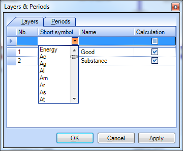
Select Layers for Calculation
Select which of the defined layers shall be considered for calculation.
- On the Edit menu, select Layers and Periods.
- On the Layers tab, in column Calculation select which layer shall be considered for calculation.
- Click OK.
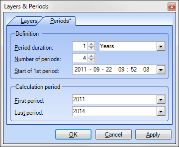
Select Periods for Calculation
Select which of the defined periods shall be considered for calculation.
- On the Edit menu, select Layers and Periods.
- On the Periods tab, select the first and the last period of the interval to be considered for calculation.
- Click OK.
Exclude Processes from Balancing (on Layer of Goods)
If only those input and output flows of process are modeled that contain a certain substance, the balancing on the layer of goods (law of material conservation, transfer coefficient equations) does not make sense. Those processes have to be marked.
- Select a process.
- On the Properties window, select the Process tab.
- Remove the tick in front of Balancing.
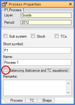
Note:
- In the system diagram, the name of processes that are not balanced during calculation on the layer of goods is written in brackets.
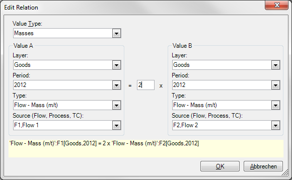
Enter Additional Linear Relations
Additional linear relation between similar data types (e.g. two flows) can be added.
- On the Edit menu, select Edit Relations.
- Click on [Enter new relation] and then
 .
.
- Choose the Value Type (e.g. Masses, Volumes, Concentrations, Transfer coefficients), Layer, Period and Source of the variables A and B.
- Define the proportion factor
- Confirm with OK.
Note:
- You can delete defined relations by clicking the relation in the list and pressing DEL.
- If relations between different layers have been defined, scaling will be switched of during calculation out of technical reasons.
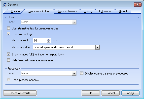
Display Coarse Balance of Processes
The coarse (mass) balance of processes (sum of known input flows minus sum of known output flows) can be displayed as a number inside of the process icons.
- On the Extras menu, select Options and click the Processes & Flows tab.
- On the Process pane, select Display coarse balance of processes.
Perform Calculation
- For a quick start of the calculation, click
 in the Data Input
toolbar or press F5.
in the Data Input
toolbar or press F5.
or
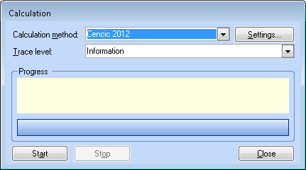
- To set additional calculation options (calculation method, trace level), choose Calculation dialog from Edit menu or press ALT + F5:
- Choose the calculation method (Cencic 2012 or IAL-IMPL2013)
- Optional: Settings to change parameters of the calculation methods. For options refer to Options Calculation Module Cencic 2012 and IAL-IMPL2013
- Optional: Choose the trace level (none < errors < warning < information < details) of logging.
- Click Start.
- After the calculation, click Close to display the results in the system diagram.
Note:
- After the calculation, in the Trace Output window, a list of information, warnings and errors is displayed. Click any entry in this list to highlight the corresponding object in the system diagram.
- The Trace Output window offers the following options:
 Show message grid
 Show text messages.
Output is dependent on trace level
Show text messages.
Output is dependent on trace level Show/Hide
Group-by-box: To group the listed messages by certain fields pull the
according column descriptions into the grey grouping area above.
Show/Hide
Group-by-box: To group the listed messages by certain fields pull the
according column descriptions into the grey grouping area above. Clear all messages
- The Degree of over-determination states how many equations without unknown variables could be found by transformation of the given equation system.
- The Value of objective function refers to the minimized value of the objective function of the weighted least squares approach used in STAN.
- The Quality of data reconciliation will be displayed if no gross errors are detected. It ranges between between 0 (i.e. the mean values of all variables contained gross errors) and 1 (i.e. the mean values of the measurements fitted perfectly and no adjustment were necessary at all).
- The Summary (histogram data) of the standard scores of the reconciled values (= (measured value - reconciled value) / standard uncertainty of measured value) is displayed.
Change Options of Calculation Module Cencic 2012
This module was developed by Oliver Cencic. It offers the following calculation options:
- Convergence tolerance: If the 2-norm of the changes in the variable vector is less than this tolerance the iterative calculation will be stopped. Default = 1E-10.
- Zero values tolerance: All absolute values less than this tolerance will be considered zero during update of vectors and matrices.
- Observability tolerance: Matrix entries (absolute) smaller than this tolerance will be considered zero during variable classification according to Madron. Default = 1E-10.
- Contradiction Check: Untick this option only if in the Trace Output window potential problems with the contradiction check are indicated.
- Short variable keys: Use short variable keys (e.g. FV:123 instead of F1_m_G_2000 to represent the mass flow of Flow 1 on the layer of goods for the period 2000) when displaying detailed results of the calculation procedure.
- Display equations: Displays used equations after computation.
Note:
- The setting of option 5 and 6, together with the chosen trace level,
influence what is displayed in the Trace Output window when
clicking .
Change Options of Calculation Module IAL-IMPL2013
This module was developed by Jeffrey Dean Kelly from Industrial Algorithms. It offers the following calculation options:
- Maximum number of non-zeros in any working matrix.
- Multiplier needed for sparse matrix operations.
- Scaling factor
- Scaling type: 0 (none), 1 (rows only), 2 (rows and columns = default), 3 (columns only).
- Gamma: A regularization parameter for B'*B to increase the numerical stability of the iterative solution especially when solving ill-conditioned systems => B'*B + gamma*Iy. Default = 1E-12.
- Epsilon: A regularization parameter for A'*Q*A + lambda*B*B' to increase the numerical stability if a row is vacuous => A'*Q*A + lambda*B*B' + epsilon*Ig. Default = 1E-12.
- Lambda: Estimated variance of the unmeasured variables used as a regularization parameter in A*Q*A' + lambda*B*B'. Default = 1E6. Will be used if no values for Lambda1 and Lambda2 are given.
- Lambda1 and Lambda2: for improved calculation of estimated raw variance of the unmeasured variables => w(i) = Lambda1 * (abs(y(i)) + Lambda2)^2. If Lambda1 or Lambda2 is less or equal 0, Lambda will be used instead. default = 100.
- Convergence tolerance: Convergence tolerance for constraint closure. If the constraint or function residuals have a 2-norm less than this tolerance then the iterative calculation is stopped.
- Zero values tolerance: All absolute values less than this tolerance will be considered zero during update of vectors and matrices.
- Observability tolerance: All entries in o.dat with an absolute value less than this tolerance will be considered zero (= observable).
- Method 1: Sparse matrix factorization technique or method used in the reconciliation solver. Valid values: 1,2,3,4
- Method 2: Sparse matrix factorization technique or method used in the post-reconciliation sensitivity solver to compute the observability and redundancy metrics. Valid values: 1,2.
Note:
-
Compared to the standard calculation algorithm Cencic 2012, IAL-IMPL 2013 is superior in calculation speed (factor 10 to 50) when dealing with large models (number of equations + variables > 4000), and offers a higher numerical stability. It operates with sparse matrices.
-
The trial-license of IAL-IMPL 2013 included in STAN is limited to a number of 200 equations + variables. If you are interested in an unlimited version, please contact Jeffrey Dean Kelly at Industrial Algorithms (jdkelly@industrialgorithms.ca) to get an unlimited 7-days-trial-license or to purchase an unlimited perpetual version for $100 (USD) for academic, non-commercial (non-consulting, non-contracting, etc.) and home use only. The price for a commercial license of IMPL can be sent upon request. The license file has to be installed by clicking Install license.
Toggle Scaling
Goal of the automatic scaling procedure is to reduce the condition number of the equation system (matrices) thus reducing the influence of disturbed input data (e.g. due to rounding errors) on the results. If scaling is not desirable or possible (e.g. use of subgood layers => scaling is switched off automatically), it can be switched off manually.
- On the Extras menu, select Options and then tab Calculation.
- Set/Delete the tick under Enable Scaling.
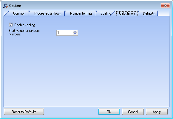
Change Initial Value of Unknown Variables
To iteratively solve non-linear equation systems, it is necessary to assign initial values to unknown variables. In STAN this procedure is performed automatically with the assistance of a random number generator. In some problems, the choice of random numbers influences the results what is not desirable. Because of that, STAN offers the possibility to change the start value of the random numbers generator, thus generating a different set of random numbers. If the calculation with different start values delivers the same results, the problem can be considered stable.
- On the Extras menu, select Options and then tab Calculation.
- Enter a value between 0 and 999 as start value for generation of random numbers.
Define Scaling Basis
- On the Model-Explorer window, click the name of the system.
- On the Properties window, enter scaling unit (e.g. capita) and scaling factor (e.g. 100.000, meaning the entered data refer to 100.000 inhabitants).
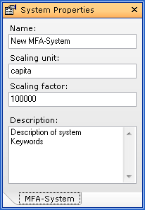
Note:
- The same settings can be edited in the Data Explorer on tab System.
- How to apply the scaling factor look at Scale Data.
Scale Data
- On the Extras menu, select Options and click the Scaling tab.
- On the Scaling pane, select the reference entity (scaling basis, sum of imports, sum of exports).
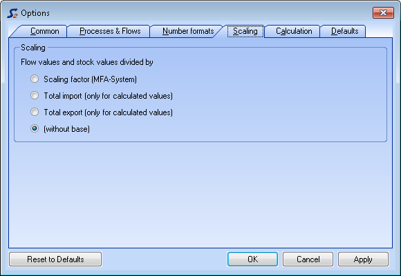
Note:
- How to define the scaling factor look at Define Scaling Basis.
Install New Calculation Modules
- On the Extras menu, click Calculation Modules.
- Click Install New Modules.
- Select the new module and click Open.
- Close the window.
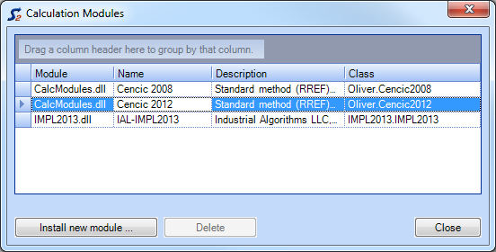
Note:
- Copy the new calculation module (extension = .dll) to the subfolder "CalcModules" in the STAN directory ".
- The existing default calculation module "CalcModules.dll" must not be removed.
- To remove installed modules requires a restart of STAN.